
In today’s post I will take a look at the Global Financial Crisis, but from a rather different perspective than how it is discussed in the media. In particular, I will use of the basic model of aggregate demand (AD) and aggregate supply (AS) to explain the changes in real GDP, CPI inflation and the unemployment rate for the United States. The data for the analysis comes from the World Development Indicators database of the World Bank.
Let’s start with a brief overview on the economic indicators of the United States in the 21st century. For this I have prepared two diagrams. Figure 1 contains the United States’ real GDP (constant 2005 US$) together with the country’s annual percentage growth rate of real GDP over the period from 2000 to 2014. The unemployment rate (ILO estimates) and inflation, as measured by the Consumer Price Index (CPI), are shown in figure 2.
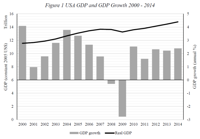
First it can be seen that the USA’s real GDP has risen steadily over the period except from 2008 and 2009, which corresponds to the GFC and the last global recession. In 2000, GDP stood at around $11.6 trillion and it has risen to $14.8 trillion in 2014. This is a 28 percent increase in real GDP over the complete period. However, despite an overall increase in GDP, GDP growth has been considerably volatile over the period. The US economy experienced the highest GDP growth in 2000 with a positive growth rate of 4.1 percent. The lowest GDP growth occurred in 2009 with a negative growth rate of 2.8 percent. This corresponds to a variation of 6.9 percentage points. The US surpassed its pre-downturn output level in 2011, meaning that it took the economy almost two years two recover from the 2008/09 recession. After the GFC, the economy has experienced more even growth from 2010 to 2014 compared to the clear rise and fall in the growth rate over the period from 2001 to 2007, which was driven by the US housing boom amongst other factors.
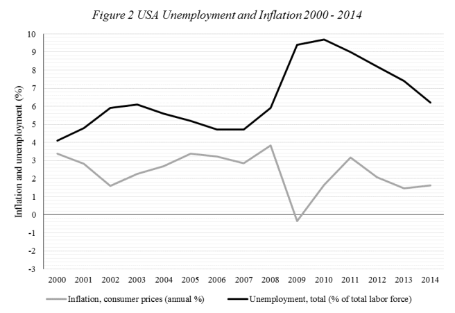
Unemployment ranged from 4.1 percent (2000) to 9.7 percent (2010) over the period from 2000 to 2014. In the beginning of the century it rose until 2003 and then fell until 2006. After stagnating in 2007 unemployment more than doubled by the end of 2010. Since then, unemployment has fallen significantly to 6.2 percent. However, this is still 1.5 percentage points higher than the pre-downturn unemployment rate.
Inflation ranged from an inflation rate of 3.8 percent in 2008 to deflation of 0.4 percent in 2009. The highest volatility in the inflation rate therefore occurred during the GFC. In the beginning of the century inflation came down to 1.6 percent (2002) and thereafter accelerated to 3.4 percent in 2005. During the period preceding the GFC it remained at a relatively high level compared to the years before. After a drop by almost 3.5 percent from 2008 to 2009 inflation receded to 3.2 percent in 2011 but it has recently dropped below the 2 percent level.
Figure 3 Supply and Demand Shock during the GFC

The fluctuations in real GDP, unemployment and inflation for the period of the GFC of 2007 can be summarized in the AS/AD model as follows (figure 3). Firstly, from 2007 to 2008 the US economy faced a negative supply shock (1) due to the collapse of a domestic housing bubble, a doubling of the oil price, as well as large price increases in other commodities (Krugman, 2009). This shifted the short run aggregate supply curve (SRAS) to the left. This negative supply shock explains the beginning of the GFC, i.e. the stagflation of 2007/08, because a negative supply shock triggers both rising inflation and lower output, as well as higher unemployment. However, this is not the end of the story, because the negative supply shock was followed by a negative demand shock in 2008/09. The aggregate demand (AD) curve also shifted to the left (2), causing disinflation in 2008 and deflation in 2009, negative output growth of almost 3 percent in 2009, as well as a further increase in the unemployment rate to almost 10 percent. It took the AD curve until 2011 to shift back to its initial position (3) as the government intervened and consumer and business confidence recovered. This caused inflation and GDP growth to pick up again as shown in figure 2. Subsequently, unemployment fell as demand recovered. Since 2011 it can be observed that unemployment and inflation are falling in tandem. This can be explained by the shifting of the SRAS curve back to its initial position (4) after the negative supply shock which occurred in 2007/08.
In sum, there are 4 shifts – 2 shifts in the AD curve and 2 shifts in the AS curve – based on the economic indicators of the US. However, it should be noted that it is a rather simplified version of the GFC story in the AS/AD model. There are certainly other factors important for explaining the GFC which are not captured in the model. Still it is great for explaining the changes in unemployment, inflation and GDP (growth). It was actually part of an assignment for one of my classes with the goal to infer from the data which of the curves in the model moved in which direction.
Many thanks for reading,
Jasse
Krugman, P., & Wells, R. (2009). Macroeconomics (2nd ed.). New York, N.Y.: Worth Publishers.
World Bank (2016). World Development Indicators: United States [Data file]. Retrieved from: http://data.worldbank.org/country/united-states
